Introduction
This self-guided course gives numeric examples of the basic calculations that a slide
rule can do. Just follow the step-by-step instructions and you will be
amazed by the power and versatility of the venerable Slipstick. Click on any of
the images below to get a large, unmarked, blowup of each slide rule as shown in
the problem.
Images created from Emulators designed by Derek Ross.
Initial examples based on Derek's Self Guided demo and expanded by Michael Konshak.
|

No Slide rule handy?
You can practice with these Virtual Slide Rule to try
these and other problems on your own. (Hint: Teachers can use a computer projector to manipulate the slide rule
in front of the class).
Want to try a real Slide Rule?
Participate in our School Loaner Program.
Sets of up to 25 slide rules are available FREE of charge for teachers to use in class.
|
A Brief Timeline of the Slide Rule
1614 - Invention of logarithms by John Napier, Baron of Merchiston,
Scotland.
1617 - Developments of logarithms 'to base 10' by Henry Briggs,
Professor of Mathematics, Oxford University.
1620 - Interpretation of
logarithmic scale form by Edmund Gunter, Professor of Astronomy, London.
1630
- Invention of the slide rule by the Reverend William Oughtred, London.
1657
- Development of the moving slide/fixed stock principle by Seth Partridge,
Surveyor and Mathematician, England.
1775 - Development of the slide rule
cursor by John Robertson of the Royal Academy.
1815 - Invention of the log
log scale principle by P.M. Roget of France.
1850 - Amédée Mannheim, France,
produced the modern arrangement of scales.
1886 - Dennert & Pape,
Germany, introduce white celluloid as a material for inscription of
scales.
1890 - William Cox of the United States patented the duplex slide rule.
c1900 - Engine divided scales on celluloid increases
precision of slide rules.
1976 - The final slide rule made by K&E donated to the Smithsonian Institute, Washington, DC,
USA.
Today, slide rules can be found on eBay, antique stores and estate auctions.
Lost inventories of brand new slide rules turn up every year.
|
Was there Life
Before Computers?
Calculations before
We Went Digital

Teaching Aid on the history of mathematics by Nicola Marras, Italy 12.5MB pdf
|
Parts of a Slide Rule


Reading the Scales
The scales on a slide rule are logarithmic, in that the spacing between divisions (the lines on the scale)
become closer together as the value increases. This is why the slide rule is able to do multiplication and division
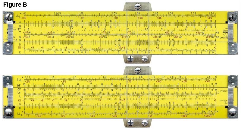
rather than addition and subtraction. Compare the two sets of offset scales
below in Figure B. In both cases the left index X:1 or C:1 is placed over the first whole
number, either Y:2 or D:2. On a linear scale the value of any number on the X
scale as read on Y is increased by 1. On a logarithmic scale, the value on any
number on the C scale as read on the D scale becomes a multiple of the number
under the index.

William Oughtred discovered the above characteristic in 1630, when he placed two
logarithmic scales that were invented by his contemporary, Edmund Gunter,
alongside each other. Thus the slide rule was born.
At this point it is best to just describe how to read the scales.
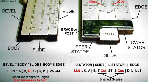
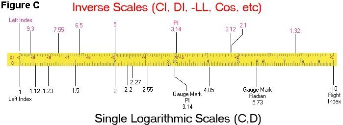
On almost all slide rules, the black scales (A, B, C, D, K, etc.) increase from left
to right. The red scales, or inverse scales
(CI, DI), increase from right to left.
The pocket sized Pickett 600-ES will be used in most illustrations. The full
sized Pickett N3-T for others. By the way, the Pickett 600-T (white) was taken by the
Apollo 11 NASA astronauts to the moon.

Except for 'folded', 'trig' or Log' scales, each scale begins
with 1. C and D scales are single logarithmic (1-10) scales. The A and B scales are double logarithmic
(1-10-100) having two cycles of 1-10,
the K scale being triple logarithmic (1-10-100-1000) having three cycles of
1-10. The Primary divisions are whole numbers.
The secondary divisions divide the Primary by 10, the Tertiary divisions divide the secondary by 5.
Of course as you get to the end of each scale the divisions get so close together that the tertiary divisions
disappear. The scales on each side of a slide rule are aligned so that
calculations can be carried from one side to the other.

Its important to become familiar with not only the physical divisions as marked on the scales, but in becoming able to
extrapolate* values when the hairline falls in the spacing between
divisions. Positions of the slide and cursor shown in the examples will mention the label of the scale
and the value on the scale, such as scale C at 1.5 will be referenced as C:1.5.
*In mathematics, extrapolation is the process of constructing new data points outside a discrete
set of known data points. It is similar to the process of interpolation,
which constructs new points between known points, but its results are often less
meaningful, and are subject to greater uncertainty (Ref: en.wickipedia.org).
Multiplication
1. Simple Multiplication (uses C and D scales)
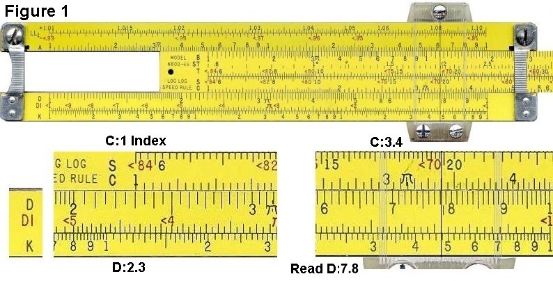
Example: calculate 2.3 × 3.4 (Figure 1)
- Slide the leftmost Index '1' on C over 2.3 on the D scale.
- Move the cursor to 3.4 on the C scale.
- The cursor is on the D scale just a bit over 7.8 or 7.82. This is the answer.

2. 'Wrap-Around' Multiplication (uses C and D scales)
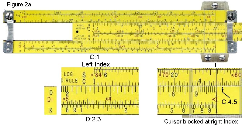
Example 2a: calculate 2.3 × 4.5 (Figure 2a)
- Move the left Index on C to 2.3 on the D scale.
- Try to move the cursor to 4.5 on the C scale. The cursor is blocked by
the brace (also called strap or bridge).
- The target C:4.5 is off the D scale. The right Index must now be used.

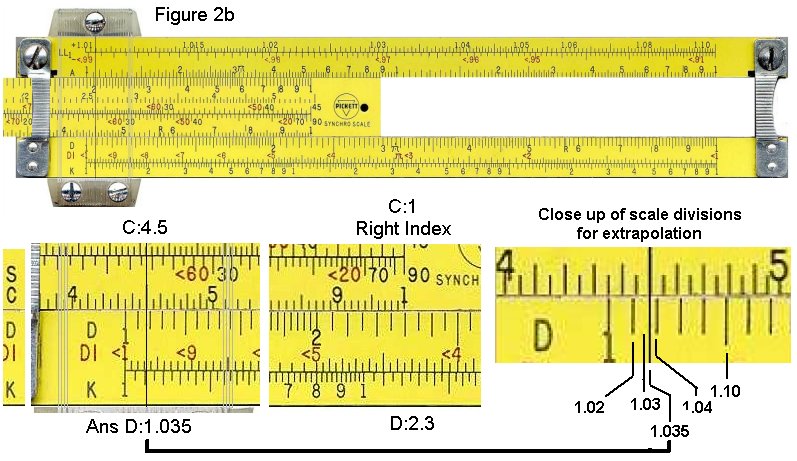
Example 2b: calculate 2.3 × 4.5 (Figure 2b)
- Move the right Index on C (C:1) to over 2.3 on the D scale (D:2.3)
- Slide the cursor to 4.5 on the C scale (C:4.5)
- On the D scale, you'll see that the hairline is between divisions.
Extrapolate the answer to 1.035.
- Do a rough approximation by rounding 2.3 to 2 and 4.5 to 5.
- We mentally calculate 2 × 5 = 10, so we
adjust the
decimal place to get 10.35 or 10.4.

3. Folded-Scale Multiplication (uses C, D, CF and DF scales)
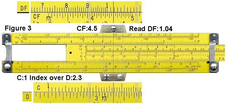
Example 3: calculate 2.3 × 4.5 (Figure 3)
- Slide the leftmost Index, '1', on C over the 2.3 on the D scale
(D:2.3).
- We can't move the cursor to 4.5 on the C scale; it's out of
range. We can use the folded scales to get this answer.
- Move the cursor to 4.5 on the CF scale (CF:4.5).
- The cursor is now at 1.04 on the DF scale (DF:1.04).
- We know the correct answer is near 2 × 5 = 10, so we
adjust the
decimal place to get 10.4.

4. Multiplication by π (uses D and DF scales)
Example 4: calculate 123 × π (Figure 4)
- Move the cursor to 1.23 on the D scale.
- The cursor is now at 3.86 on the DF scale.
- We know that the correct answer is near 100 × 3 = 300, so
we
adjust the decimal place to get 386.

Division
5. Simple Division (uses C and D scales)
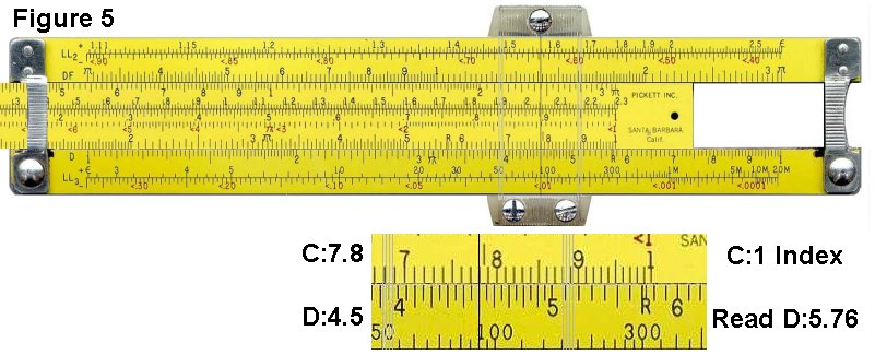
Example 5: calculate 4.5 / 7.8 (Figure 5)
- Move the cursor to 4.5 on the D scale.
- Slide 7.8 on the C scale to the cursor.
- Move the cursor to either the leftmost or rightmost '1' on the C
scale, whichever is in range. In this case, you would move it to the
rightmost '1'.
- The cursor is now at 5.76 on the D scale.
- We know that the correct answer is near 4/8 = 0.5, so we adjust
the decimal place to get 0.576.

6. Reciprocal (uses C and CI scales)
Example 6: calculate the reciprocal of 7.8, or 1/7.8 (Figure 6)
- Move the cursor to 7.8 on the CI scale. Note that the CI scale
increases from right to left, as indicated by the '<' symbols before
the numbers.
- The cursor is now at 1.28 on the C scale.
- We know that the correct answer is near 1/10 = 0.1, so we adjust
the decimal place to get 0.128.

Trigonometry
7. Sin(x) for angles between 5.7° and 90° (uses S and C scales)
Example 7: calculate sin(33°) (Figure 7)
- Move the cursor to 33 on the S scale.
- The cursor is at 5.45 on the C scale.
- We know that the correct answer for a sin in this range is
between 0.1 and 1, so we adjust the decimal place to get 0.545.

8. Cos(x) for angles between 5.7° and 90° (uses S and C scales)
Example 8: calculate cos(33°). (Figure 8)
- The cos scale shares the sin S scale. Instead of increasing
from left to right like the sin scale, cos increases from right to
left. This is indicated on the slide rule by '<' characters which
remind you that the number in increasing 'backwards'.
- Move the cursor to <33 on the S scale.
- The cursor is now at 8.4 on the C scale.
- We know that the correct answer for a cos in this range is
between 0.1 and 1, so we adjust the decimal place to get 0.84.

9. Tan(x) for angles between between 5.7° and 45° (uses T and C scales)
Example 9: calculate tan(33°) (Figure 9).
- Move the cursor to 33 on the T scale.
- The cursor is now at 6.5 on the C scale.
- We know that the correct answer for a tan in this range is
between 0.1 and 1, so we adjust the decimal place to get 0.65.

10. Tan(x) for angles between between 45° and 84° (uses backward T and CI scale)
Example 10a: calculate tan(63°) (Figures 10a and 10b)
- Move the cursor to <63 on the T scale. Note that this range
increases from right to left, as indicated by the '<' before the
numbers.
- The cursor is now at <1.96 on the DI scale. Figure 10a
- If you flip to the other side the cursor is also at <1.96 on the
CI scale. Figure 10b
- We know that the correct answer for a tan in this range is
between 1 and 10, so we don't need to adjust the decimal place.


11. Tan(x) for angles between between 45° and 84° (uses forward T and C scale)
Example 11: calculate tan(63°). (Figure 11)
- Move the cursor to 63 on the forward T scale. This scale
increases from left to right.
- The cursor is now at 1.96 on the C scale.
- We know that the correct answer for a tan in this range is
between 1 and 10, so we don't need to adjust the decimal place.

12. Sin(x) and tan(x) for angles between 0.6° and 5.7° (using the ST and C scales)
In this range, the sin and tan functions are very close in value, so a
single scale can be used to calculate both.
Example: calculate sin(1.5°) (Figure 12)
- Move the cursor to 1.5 on the ST scale.
- The cursor is now at 2.62 on the C scale.
- We know that the correct answer for a sin in this range is
between 0.01 and 0.1, so we adjust the decimal place to get 0.0262.

13. Sin(x) and tan(x) for other small angles (using C and D scales)
For small angles, the sin or tan function can be approximated closely
by the equation:
sin(x) = tan(x) = x / (180/π) = x / 57.3.
Knowing this, the calculation becomes a simple division. This technique
can also be used on rules without an ST scale.
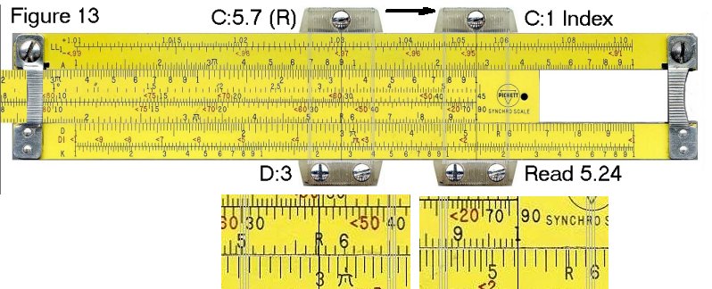
Example: calculate sin(0.3°) (Figure 13)
- Move the cursor to 3 on the D scale.
- Slide 5.73 on the C scale to the cursor. Most rules have a tick
labeled 'R' at this point.
- Move the cursor to either the leftmost or rightmost '1' on the C
scale, whichever is in range.
- The cursor is now at 5.24 on the D scale.
- We know that the correct answer is near 0.3 / 60 = 0.005, so we
adjust the decimal place to get 0.00524.

Squares and Square Roots
14. Square (uses C and B scales)
Example 14: calculate 4.7 2
- Move the cursor to 4.7 on the C scale.
- The cursor is now at 2.2 on the B scale.
- We know that the correct answer is near 52 = 25, so we
adjust the decimal place to get 22.

15. Square Root (uses C and B scales)
Example 15a: calculate √4500 (Figure 15)
- You will notice that the B scale has two similar halves. The
first step is to decide which half to use to find a square root.
- The left half is used to find the square root of numbers with odd
numbers of digits or leading zeros after the decimal point. The right
half is used for numbers with even numbers of digits or leading zeros.
Since 4500 has an even number of digits, then we'll use the right half
of the scale.
- Move the cursor to 4.5 on the right half of the B scale.
- The cursor is now at 6.7 on the C scale.
- We know that 702 = 4900, which is in the ballpark of
4500. Therefore we adjust the decimal point to get a result of 67.

Example 15b: calculate √450 (Figure 15b)
- Try it a again with a three digit number.
- Move the cursor to 4.5 on the left half of the B scale.
- The cursor is now at 2.12 on the C scale.
- We know that 202 = 400, which is in the ballpark of
450. Therefore we adjust the decimal point to get a result of 21.2

Cubes and Cube Roots
16. Cube (uses D and K scales)
Example 16: calculate 4.73 (Figure 16)
- Move the cursor to 4.7 on the D scale.
- The cursor is now at 1.04 on the K scale.
- We know that the correct answer is near 5 x 5 x 5, which, to
further approximate, is near 5 x 5 x 4 = 5 x 20 = 100. Therefore we
adjust the decimal point to get a result of 104.

17. Cube Root (uses D and K scales)
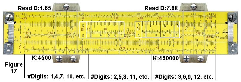
Example 17a: calculate 3√4500 (Figure 17 - left)
- You will notice that the K scale has three similar thirds. The
first step is to determine which third to use to find the cube root.
- The first third is used to find the cube root is numbers with one
digit. You can cycle through the thirds, increasing the number of
digits by one
for each third, to find which part to use. Just like having a line of people and you count off into 3's.
- For the value of 4500, which has 4 digits, we cycle through the
thirds and find that we would use the first third.
- Move the cursor to 4.5 on the first third of the K scale.
- The cursor is now at 1.65 on the D scale.
- We can take a guess that the correct answer is around 10. The
cube of 10 is 1000 and the cube of 20 is 8000. Thus we know that the
correct answer is between 10 and 20, therefore we can move the decimal
place and get the correct result of 16.5.

Example 17b: calculate 3√450000 (Figure 17 - right)
- For the value of 450000, which has 6 digits, we cycle through the
thirds and find that we would use the third third.
- Move the cursor to 4.5 on the third third of the K scale.
- The cursor is now at 7.68 on the D scale.
- We can take a guess that the correct answer is around 10. The
cube of 10 is 1000 and the cube of 100 is 1000000. Thus we know that the
correct answer is between 10 and 100, therefore we can move the decimal
place and get the correct result of 76.8.
Log-Log Scales
Log-log scales are used to raise numbers to powers. Unlike many of the
other scales, log-log scales can't be learned simply be memorizing a
few
rules. It is necessary to actually understand how they work. These
examples are intended to gradually introduce you to the concepts of
log-log scales, so you gain that understanding. Hopefully, the power of
10 examples don't bore you, as they lay the foundation for later
examples.
Since there are many slight variations of log-log scales on different
slide rules, I'll refer only to the scales found on the Pickett N3,
Pickett N600 and Pickett N803 slide rules (among others). If you want
to view a virtual N3, click here,
if you want a virtual N600, click here
(opens in a new window.)
Another interesting aspect of LL scales is that the decimal point
is "placed." That is, you don't have to figure out afterwards where the
decimal point belongs in your result. The disadvantage to this is that
LL scales are limited in the numbers they can calculate. Typically, the
highest result you can get is about 20,000, and the lowest is 1/20,000
or 0.00005. One exception to this is the Picket N4 (virtual here),
which goes up to 1010.
18. Raising a Number to Powers of 10 (N>1)
To raise a number to the power of 10, simply move the cursor to the
number and look at the next highest LL scale. (These examples are for
numbers greater than 1. )
Example 18a: calculate 1.35 10 (uses LL2
and
LL3 scales) (Figure 18a)
- Move the cursor to 1.35 on the LL2 scale.
- The cursor is at 20.1 on the LL3 scale. This is the correct
answer.

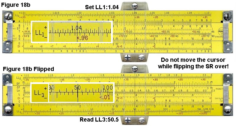
Example 18b: calculate 1.04 100 (uses LL1
and
LL3 scales) (Figure 18b)
- Set the cursor over 1.04 on the LL1 scale.
- Flip the SR over
(on some advanced SR's the LL0, LL1, LL2 and LL3 will be on the same side)
- The cursor is at 50.5 on the LL3 scale.

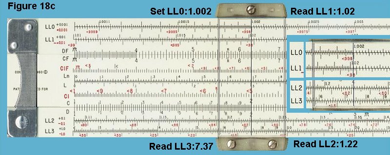
Example 18c: calculate 1.002 1000 (uses LL0 and LL3
scales) (Figure 18c)
- Set the cursor over 1.002 on the LL0 scale.
- The cursor is on 7.4 on the LL3 scale. This is the correct answer.

Example 18d: calculate sequential powers of ten of 1.002 (uses LL0, LL1, LL2 and
LL3
scales) (use the above Figure 18c)
- Set the cursor to 1.002 on the LL0 scale. This the same as 1.002 1
- On LL1, the cursor is at 1.002 10 , or 1.020
- On LL2, the cursor is at 1.002 100 , or 1.22.
- On LL3, the cursor is at 1.002 1000 , or 7.37.
19. Raising a Number to Powers of 10 (N<1)
The reciprocals of the LL scales are the -LL scales. They work the same
way, but you have to make sure that you look for the answer on a -LL
scale. They are RED scales so they increase in
value from right to left.
Example 19: calculate 0.75 10 (uses
-LL2
and -LL3 scales)
- Move the cursor to <0.75 on the -LL2 scale.
- The cursor is at <0.056 on the -LL3 scale. This is the correct
answer.

20. Raising a Number to Powers of -10 (N<1), N-10 or 1/N10
The reciprocals of the LL scales are the -LL scales. They work the same
way, but you have to make sure that you look for the answer on a -LL
scale.
Example 20: calculate 1.175 -10 (uses
LL2
and -LL3 scales)
- Set the cursor hairline to 1.175 on the LL2 scale.
- The hairline is over 5 on the LL3 scale. This is 1.175 10
- The cursor is also over .2 on the -LL3 scale. This is the reciprocal of 1.175 -10 or 1/1.175 10 and is the correct
answer.

21. Finding the 10th Root (N>1)
As you've seen in the previous examples, to raise a number to the 10th
power, you simply look at the adjacent number on the next highest LL
scale. To find a tenth root, you look at the adjacent number on the
next lowest LL scale. Remember also that finding the tenth root is the
same as raising a number to the power of 0.1.
Example 21: calculate 10√5, or 5 0.1
(uses LL2 and LL3 scales) (Figure 21)
- Set the cursor over 5 on the LL3 scale.
- The cursor is now at 1.175 on the LL2 scale. This is the correct
answer.

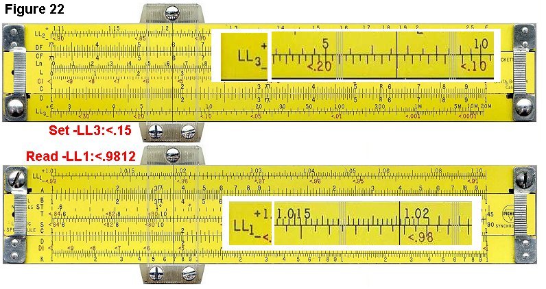
22. Finding the 10th Root (N<1)
Example: calculate 100√0.15, or 0.15 0.01
(uses -LL3 and -LL1 scale) (Figure 22)
- Set the cursor to 0.15 on the -LL3 scale.
- Flip the SR to the other side to read the LL1 scale.
- The cursor reads 0.9812 on the -LL1 scale. This is the
correct answer.

23. Arbitrary Powers (Staying on Same LL Scale)
Occasionally, depending on the numbers, it is possible to calculate a
power without switching scales.
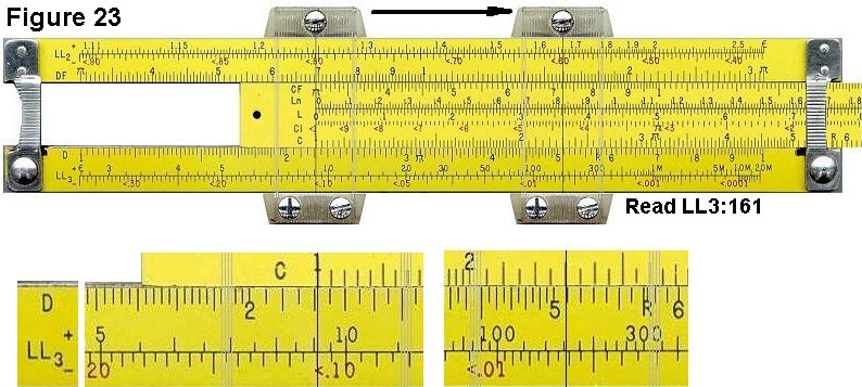
Example: calculate 9.1 2.3
(uses LL3 scale) (Figure 23a)
- Set the cursor hairline to 9.1 on the LL3 scale.
- Slide the leftmost Index '1' on C to the hairline.
- Move the hairline over 2.3 on the C scale.
- The cursor is now at about 161 on the LL3. This is very close to
the correct answer of 160.6. One of the problems with LL scales is that
their accuracy diminishes as the numbers increase in value.

Example: calculate 230 0.45 (uses
LL3 and C scale) (Figure 23b)
- Set the cursor to 230 on the LL3 scale.
- Since we're raising to a power that's less than 1, we have to go
left on the LL scale.
- Slide the rightmost Index '1' on the C scale to the cursor hairline.
- Move the cursor to 4.5 on the C scale.
- The cursor is now at 11.6 on the LL3 scale. This is close to the
correct answer of 11.56.
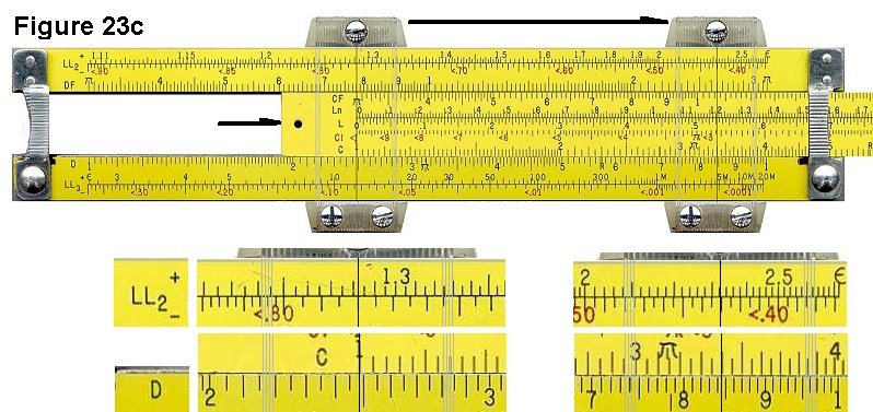
 Example: calculate 0.78 3.4 (uses -LL2 and C scale)
(Figure 23c)
- Set the cursor to 0.78 on the -LL2 scale.
- Slide the leftmost Index '1' on the C scale to the cursor hairline.
- Move the cursor to 3.4 on the C scale.
- The cursor is now at 0.43 on the -LL2 scale. This is the correct
answer.
 Try another:
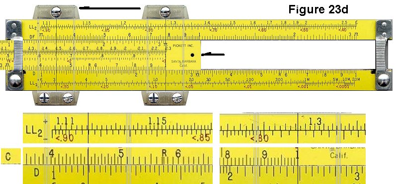
Example: calculate 0.78 0.45 (uses -LL2 and C scale) (Figure 23d)
- Set the cursor to 0.78 on the -LL2 scale.
- Since we're raising to a power that's less than 1, we have to go
left on the LL scale.
- Slide the rightmost Index '1' on the C scale to the cursor hairline.
- Move the cursor to 4.5 on the C scale.
- The cursor is now at 0.894 on the -LL2 scale. This is the correct
answer.

24. Arbitrary Powers (Switching LL Scales)
One of the rules of exponents is that (A B ) C
is equal to A B x C. We can use this fact, along with our
knowledge of powers of ten, to calculate arbitrary powers.
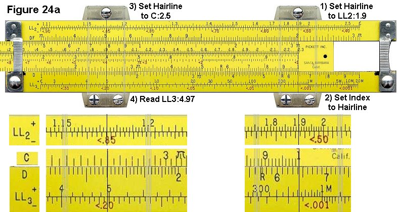
Example: calculate 1.9 2.5
(uses LL2, C and LL3 scales) (Figure 24a)
- If we try to calculate this the easy way, the power 2.5 is out of
range for the scale.
- We can reinterpret the problem as:
Calculate (1.9 0.25 ) 10
Because 0.25 x 10 is 2.5.
- Set the cursor hairline to 1.9 on the LL2 scale.
- Slide the rightmost Index '1' on the C scale to the hairline.
- Shift the cursor hairline to 2.5 on the C scale.
- The hairline is now at 1.9 0.25 on the LL2 scale. Since
we want to also raise this to the power of 10, we look "one scale
higher" at the LL3 scale.
- The cursor is at 4.97 on the LL3 scale. This is the correct
answer.
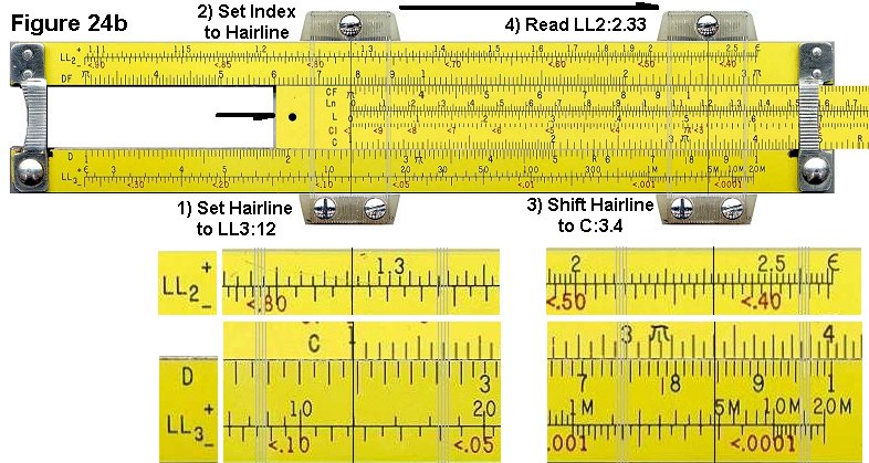
 Example: calculate 12 0.34 (uses
LL3, C and LL2 scales) (Figure 24b)
- Like the previous example, if we try to calculate this the easy
way, the power 0.34 is out of range for the scale.
- We can reinterpret the problem as:
Calculate (12 3.4 ) 0.1
Because 3.4 x 0.1 is 0.34.
- Move the cursor to 12 on the LL3 scale.
- Slide the leftmost '1' on the C scale to the cursor.
- Move the cursor to 3.4 on the C scale.
- The cursor is now at 12 3.4 on the LL3 scale, which
is about 5000 (which is not the number we're looking for). Since we
also want to raise this to the power of 0.1, we look at the LL2 scale.
- The cursor is now at 2.33 on the LL2 scale. This is the correct
answer.
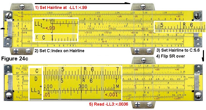
 Example: calculate 0.99 560 (uses -LL1, C and
-LL3 scales) (Figure 24c)
- We can reinterpret this problem as:
Calculate (0.99 5.6 ) 100
Because 5.6 x 100 = 560
- Set the cursor Hairline to <0.99 on the -LL1 scale.
- Shift the leftmost Index '1' on the C scale to the cursor hairline.
- Move the cursor to 5.6 on the C scale.
- The cursor is now at <0.99 5.6 = <.9452
on the -LL1 scale.
-
Since we also want to raise this to the power of 100, we look "two
scales higher", or the -LL3 scale.
- The cursor is now at <0.0036 on the -LL3
scale. This is the
correct answer.

25. Log-Log Approximations
In general, LL scales don't handle numbers extremely close to 1, such
as 1.001 or 0.999. This is not a problem because there is an accurate
approximation for numbers in this range. In general, if you have a very
small number 'd', then:
(1 + d) p = 1 + d p
Example: calculate 1.00012 34 (uses C and D scales) (Figure
25a)
- In this case, if we use the approximation (1 + d) p =
1 + d p, then:
d = 0.00012, and
p = 34
- We must calculate 0.00012 * 34.
- Set the leftmost Index '1' on the C scale to 1.2 on the D scale..
- Set the cursor hairline on 3.4 on the C scale.
- The cursor is now at 4.08 on the D scale.
- We know that the correct answer would be near 0.0001 * 30, or
0.003. Therefore we adjust the decimal point to get a value of 0.00408.
- Add 1 to 0.00408. The result is 1.00408, which is very close to
the correct answer of 1.004088.
 Example: calculate 0.99943 21 (uses C and D
scales) (Figure 25b)
- Like before, we'll use the approximation (1 + d) p =
1 + d p. In this case:
d = (0.99943 - 1) = -0.00057, and
p = 21
- We must calculate -0.00057 * 21.
- Slide the rightmost Index '1' on the C scale to 5.7 on the D scale.
- Move the cursor hairline over 2.1 on the C scale.
- The hairline is at 1.195 on the D scale.
- We know that the correct answer would be near -0.0006 * 20, or
-0.0120. Therefore we adjust the decimal point to get a value of
-0.01195.
- Subtract 0.01195 from 1. The result is (1 - 0.01195) = 0.98803.
This is very close to the correct answer of 0.98809.

ISRM Slide Rule Loan Program
If you are an educator or home schooler wishing to give your students a hands-on experience and instruction with
actual slide rules, the museum is able to supply quantities of up to 25 matching slide rules for temporary use, free of charge, to many countries, courtesy of several collectors and members of the Oughtred Society, Dutch Kring, and German RST. Find out more about it here.
Additional Resources
Instructions, Manuals, Scales and Construction
You can download additional instructions from the
ISRM museum library
or visit one of the following sites.
In the beginning, at the time of the great flood, Noah went thru his ark after it landed, and found two small snakes huddled in a corner. Noah looked at these poor specimens - and said "I told you to go forth and multiply - why haven't you?"
The poor snakes looked up at Noah and replied "We can't because we are adders....."
Noah looked a bit perplexed, and then proceeded to tear bits of planking from his ark. He went on to build a beautiful wooden platform. He gathered up the snakes and placed them on the platform, and joyfully told the snakes - "Now go forth and multiply, because even adders can multiply on a log table"
D. Scott MacKenzie, PhD
Metallurgist specializing in Heat Treatment and Quenching
Example set Copyright © 2005 Derek Ross.
Modifications, layout and graphics Copyright © 2006 by Michael V. Konshak
|
|


